# init repo notebook
!git clone https://github.com/rramosp/ppdl.git > /dev/null 2> /dev/null
!mv -n ppdl/content/init.py ppdl/content/local . 2> /dev/null
!pip install -r ppdl/content/requirements.txt > /dev/null
!pip install rlxutils > /dev/null
import numpy as np
import matplotlib.pyplot as plt
from scipy import stats
from scipy.integrate import quad, dblquad
from rlxutils import subplots
import daft
import seaborn as sns
import pandas as pd
from progressbar import progressbar as pbar
from itertools import product
import tensorflow_probability as tfp
import tensorflow as tf
tfd =  tfp.distributions

%matplotlib inline
Scenarios with Bayes#
Remember Bayes theorem:
and recall that this is a relation between marginal, conditional and joint probability distributions.
Bayes’ theorem does not make any assumption on how the different probabilities come into existance and, thus, it can be used and interpreted in many different scenarios:
independence of measurements: we are given two clinical variables of patients (cholesterol and age), which may, or may not be correlated, but there is no temporality or causality initally associated between then, both can be measured at any time regardless the other.
time dependance: we consider \(z\) happens (or is measured) before \(x\), such as when modelling causality (I aim a gun and then I shoot).
latent variables: we consider \(z\) a latent variable that explains or generates \(x\) an observed variable.
of course, each scenario comes with its limitations. Normally \(p(x)\) is intractable or very difficult to compute, etc.
We will call the different terms of Bayes theorem this way (with analogies on the time dependance example above):
\(p(z)\): the prior, our initial knowledge or assumption of how \(z\) is distributed. This would be our estimation on how do I aim a gun (like a distribution of directions in which I generally aim with respect to a target).
\(p(x)\): the evidence, what we observe. The positions in the target where my shots hit.
\(p(x|z)\): the model, the probability of seeing \(x\) is we assume a certain value of \(z\). A model which, giving an aiming direction \(z\), produces a probability distribution of possible positions of where would my shot hit the target. This would take into account the gravity, distance, direction, etc. \(p(x|z)\) is a result of applying Newton’s laws to \(z\) and the shooting conditions.
\(p(z|x)\): the posterior. Given an observation \(x\), what possible aiming directions could have produced it.
Models and goals#
In general we are given data (observations of \(x\), and possibly of \(z\)) and we will be asked for the posterior. But the posterior might have different meanings in different settings. It is key to understand what question you are answering we you are asked to get the posterior:
independance of measurements: \(x\) is cholesterol, \(x\) is age. If I make an observations of \(x\), the posterior \(p(z|x)\) is answering the question In what ages is more typical this observation cholesterol?
causality: \(z\) is my aiming direction, \(x\) is the position in the target where my shot hit. If I make an observation \(x\), the posterior \(p(z|x)\) is answering the question What possible aiming conditions could have produced this shot mark in the target?
In different problem settings we might be given different things, and need to obtain others. For instance
given one observation \(x_i\), \(p(z)\) and \(p(x|z)\) obtain \(p(z|x_i)\), this is, the posterior for that specific observation. And there will be choices in what tools, methods or data to use, but not on the shape or properties on the different distributions.
given many observations, \(p(z)\) and \(p(x|z)\) obtain a function that computes \(p(z|x)\) for any observation.
give one or many observations and only \(p(z)\) design a parametrized version of \(p(x)\), \(p(x|z)\) and \(p(z|x)\), and try to obtain the parameters that best fit the data. This will be the case of the variational autoencoder.
Computing vs designing#
Observe the subtlety between the statements above.
When asked to obtain something we have no design choices. Obtaining typically refers to computing some result with a higher or lower degree of generality. This might be challenging for many reasons: intractability, numerical instabilities, hard to implement, lack of tools, etc.
When asked to design something we make choices that imply different trade-offs. For instance, a variational autoencoder designs a setting in which \(p(x|z)\), \(p(z|x)\), \(p(z)\) and \(p(x)\) have certain desirable properties.
See the chain sampling process below to follow up the discussion on this.
Single observation posterior with model#
we have an scenario where we are given:
\(p(z)\), the prior
\(p(x|z)\), a model
We observe one \(x\) and we are asked to obtain \(p(z|x)\), the posterior. Our answer must be a distribution (not a number). This is a scenario in which we are asked to obtain something, there are no design choices about the distributions here. However, this is in general a dificult question, and we might restrict the possible solutions that we produce to make it easier.
This may correspond to an scenario where we are given a model on how \(x\) is generated from \(z\).
For instance, given a level of acidity of a liquid (\(z\)), we have a stochastical model that gives us the distribution of energies that we would get in a chemical reaction (\(x\)). This model is \(p(x|z)\). This model has been tested and is given to us.
We use JointDistributionSequential to model \(p(z)\) and \(p(x|z)\)
analytical or numerical solutions for all distributions#
in theory with \(p(z)\) and \(p(x|z)\) we could obtain the rest of distributions:
but this is normally not possible and thus, we need to resort to MCMC, Variational Inference, etc.
In this case, since it is a simple scenarion with known 1D variables, we can solve or compute the distributions above.
class Scenario:
def __init__(self):
self.zx_joint = self.get_joint()
self.z_samples, self.x_samples = self.zx_joint.sample(10000)
self.zmin, self.zmax = np.min(self.z_samples), np.max(self.z_samples)
self.xmin, self.xmax = np.min(self.x_samples), np.max(self.x_samples)
self.zr = np.linspace(self.zmin, self.zmax, 100)
self.xr = np.linspace(self.xmin, self.xmax, 100)
self.dz = self.zr[1] - self.zr[0]
self.dx = self.xr[1] - self.xr[0]
self.pzx = self.zx_joint.prob
self.pz = lambda z: self.zx_joint.submodules[0].prob(z) # from the joint sequential distribution
self.px = lambda x: tf.experimental.numpy.nansum(self.pzx(self.zr,x))*self.dz # numerical integration using the rectangle rule
self.pz_given_x = lambda z,x: self.pzx(z,x)/self.px(x) # joint sequential plus numerical integratin
self.px_given_z = lambda x,z: self.pzx(z,x)/self.pz(z) # joint sequential only
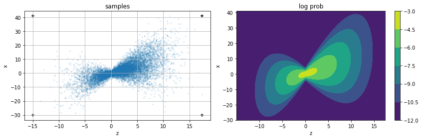
def plot(self):
for ax,i in subplots(2, usizex=6, usizey=4):
if i==0:
plt.scatter(self.z_samples, self.x_samples, alpha=.1, s=5)
plt.scatter([self.zmin, self.zmin, self.zmax, self.zmax], [self.xmin, self.xmax, self.xmin, self.xmax], marker="+", color="black")
plt.grid()
plt.xlabel("z"); plt.ylabel("x");
plt.title("samples")
if i==1:
zxgrid = np.r_[list(product(self.xr, self.zr))]
pzxgrid = self.pzx(zxgrid[:,1],zxgrid[:,0]).numpy().reshape(len(self.xr), len(self.zr))
plt.contourf(self.zr,self.xr,np.log(pzxgrid+1e-5))
plt.colorbar();
plt.title("log prob")
plt.xlabel("z"); plt.ylabel("x");
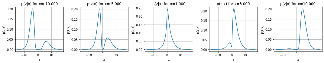
def plot_pz_given_x(self, xis):
for ax,i in subplots(len(xis)):
plt.plot(self.zr, self.pz_given_x(self.zr,xis[i]))
plt.title(f"p(z|x) for x={xis[i]:.3f}")
plt.xlabel("z")
plt.ylabel("p(z|x)")
plt.grid()
def plot_pz_given_xi(self, observed_xi, n_samples=5000):
"""
for a given observation:
- take one sample zi from p(z|xi)
- take one sample xhati from p(x|zi)
- do many times
plot histogram of xhati
"""
pz_given_xi = self.pz_given_x(self.zr,observed_xi).numpy()
# sample from p(z|xi)
pz_given_xi_sample = [self.zr[np.argwhere(pz_given_xi.cumsum()*self.dz>np.random.random())[0][0]] for _ in range(10000)]
# sample from p(x|zi)
xh_sample = []
for _ in pbar(range(5000)):
_z = np.random.choice(pz_given_xi_sample)
pxh_given_z = self.px_given_z(self.xr, _z).numpy()
cumsum = pxh_given_z.cumsum()*self.dx
rnd = np.random.random() * cumsum[-1]
_x = self.xr[np.argwhere(cumsum>rnd)[0][0]]
xh_sample.append(_x)
for ax,i in subplots(2, usizex=5, usizey=4):
if i==0:
plt.plot(self.zr, pz_given_xi, color="black")
plt.hist(pz_given_xi_sample, bins=100, alpha=.5, density=True);
plt.title(f"$p(z|x_i)$ for $x_i=${observed_xi:.3f}")
plt.xlabel("z")
plt.grid();
if i==1:
plt.hist(xh_sample, density=True, bins=100, alpha=.5);
plt.axvline(observed_xi, color="black", label="observed $x_i$")
plt.title("distribution of $\hat{x}$\nobtained by sampling $z_i \sim p(z|x_i)$ and then $\hat{x}_i \sim p(x|z_i)$")
plt.legend()
plt.grid();
plt.xlabel("x");
class ScenarioMultiModal(Scenario):
def get_joint(self):
return tfd.JointDistributionSequential([
tfd.Normal(loc=2, scale=4),
lambda z: tfd.Normal(loc=z, scale=tf.math.abs((z))*1+1)
], batch_ndims=0)
class ScenarioDependantGaussian(Scenario):
def get_joint(self):
return tfd.JointDistributionSequential([
tfd.Normal(loc=1, scale=4),
lambda z: tfd.Normal(loc=z, scale=4.)
], batch_ndims=0)
class ScenarioIndependantGaussian(Scenario):
def get_joint(self):
return tfd.JointDistributionSequential([
tfd.Normal(loc=1, scale=4),
lambda z: tfd.Normal(loc=3+0.00001*z, scale=4.)
], batch_ndims=0)
scenario = ScenarioDependantGaussian()
scenario = ScenarioMultiModal()
scenario.plot()
scenario.plot_pz_given_x(xis = [-10, -5,1,3,10])
Chain sampling#
We do the following process
Make one observation \(x_i\)
Take one sample \(z_i\) from \(p(z|x_i)\)
Take one sample \(\hat{x}_i\) from \(p(x|z_i)\)
Go to 2 many times
We will endup with a bunch of samples \(\hat{x}\). In general, in this scenario (there are no design choices), there is no particular relation between \(x_i\) and the distribution of \(\hat{x}\). You can see that in the experiment below.
When we will see the variational autoencoders, we will see that \(p(x|z)\) and \(p(z|x)\) are designed so that \(x_i\) is the MLE of \(\hat{x}\) and we can reconstruct input data from the distributions of latent variables.
In the experiment below we use Inverse Transform Sampling by using the numerical CDF of each distribution.
observed_xi=-5
scenario.plot_pz_given_xi(observed_xi = -5)
10% (530 of 5000) |## | Elapsed Time: 0:00:09 ETA: 0:01:32
---------------------------------------------------------------------------
KeyboardInterrupt                         Traceback (most recent call last)
<ipython-input-29-1e135e60a696> in <module>
----> 1 scenario.plot_pz_given_xi(observed_xi = -5)

<ipython-input-3-872f987b159a> in plot_pz_given_xi(self, observed_xi, n_samples)
     64     for _ in pbar(range(5000)):
     65         _z = np.random.choice(pz_given_xi_sample)
---> 66         pxh_given_z = self.px_given_z(self.xr, _z).numpy()
     67         cumsum = pxh_given_z.cumsum()*self.dx
     68         rnd = np.random.random() * cumsum[-1]

<ipython-input-3-872f987b159a> in <lambda>(x, z)
     18
     19       self.pz_given_x = lambda z,x: self.pzx(z,x)/self.px(x) # joint sequential plus numerical integratin
---> 20       self.px_given_z = lambda x,z: self.pzx(z,x)/self.pz(z) # joint sequential only
     21
     22   def plot(self):

/usr/local/lib/python3.7/dist-packages/tensorflow_probability/python/distributions/joint_distribution.py in prob(self, *args, **kwargs)
    917     """
    918     name = kwargs.pop('name', 'prob')
--> 919     return self._call_prob(self._resolve_value(*args, **kwargs), name=name)
    920
    921   # Override the base method to capture *args and **kwargs, so we can

/usr/local/lib/python3.7/dist-packages/tensorflow_probability/python/distributions/distribution.py in _call_prob(self, value, name, **kwargs)
   1326         return self._prob(value, **kwargs)
   1327       if hasattr(self, '_log_prob'):
-> 1328         return tf.exp(self._log_prob(value, **kwargs))
   1329       raise NotImplementedError('prob is not implemented: {}'.format(
   1330           type(self).__name__))

/usr/local/lib/python3.7/dist-packages/tensorflow_probability/python/distributions/joint_distribution.py in _log_prob(self, value)
    678   def _log_prob(self, value):
    679     return self._reduce_log_probs_over_dists(
--> 680         self._map_measure_over_dists('log_prob', value))
    681
    682   def _unnormalized_log_prob(self, value):

/usr/local/lib/python3.7/dist-packages/tensorflow_probability/python/distributions/joint_distribution.py in _map_measure_over_dists(self, attr, value)
    748         seed=samplers.zeros_seed(),
    749         sample_and_trace_fn=(
--> 750             lambda dist, value, **_: ValueWithTrace(value=value,  # pylint: disable=g-long-lambda
    751                                                     traced=attr(dist, value))))
    752

/usr/local/lib/python3.7/dist-packages/tensorflow_probability/python/distributions/joint_distribution.py in _call_execute_model(self, sample_shape, seed, value, sample_and_trace_fn)
    853       return self._execute_model(
    854           sample_shape=sample_shape, seed=seed, value=flat_value,
--> 855           sample_and_trace_fn=sample_and_trace_fn)
    856
    857     # Set up for autovectorized sampling. To support the `value` arg, we need to

/usr/local/lib/python3.7/dist-packages/tensorflow_probability/python/distributions/joint_distribution.py in _execute_model(self, sample_shape, seed, value, stop_index, sample_and_trace_fn)
   1054         if stop_index is not None and index == stop_index:
   1055           break
-> 1056         d = gen.send(next_value)
   1057     except StopIteration:
   1058       pass

/usr/local/lib/python3.7/dist-packages/tensorflow_probability/python/distributions/joint_distribution_sequential.py in _model_coroutine(self)
    390     xs = []
    391     for dist_fn, args in zip(self._dist_fn_wrapped, self._dist_fn_args):
--> 392       dist = dist_fn(*xs)
    393       if not args:
    394         dist = self.Root(dist)

/usr/local/lib/python3.7/dist-packages/tensorflow_probability/python/distributions/joint_distribution_sequential.py in dist_fn_wrapped(*xs)
    601           '(dist_fn: {}, expected: {}, saw: {}).'.format(
    602               i, dist_fn, len(args), len(xs)))
--> 603     return dist_fn(*reversed(xs[-len(args):]))
    604   return dist_fn_wrapped, args
    605

<ipython-input-3-872f987b159a> in <lambda>(z)
     90         return tfd.JointDistributionSequential([
     91             tfd.Normal(loc=2, scale=4),
---> 92             lambda z: tfd.Normal(loc=z, scale=tf.math.abs((z))*1+1)
     93         ], batch_ndims=0)
     94

<decorator-gen-329> in __init__(self, loc, scale, validate_args, allow_nan_stats, name)

/usr/local/lib/python3.7/dist-packages/tensorflow_probability/python/distributions/distribution.py in wrapped_init(***failed resolving arguments***)
    340       # called, here is the place to do it.
    341       self_._parameters = None
--> 342       default_init(self_, *args, **kwargs)
    343       # Note: if we ever want to override things set in `self` by subclass
    344       # `__init__`, here is the place to do it.

/usr/local/lib/python3.7/dist-packages/tensorflow_probability/python/distributions/normal.py in __init__(self, loc, scale, validate_args, allow_nan_stats, name)
    144           allow_nan_stats=allow_nan_stats,
    145           parameters=parameters,
--> 146           name=name)
    147
    148   @classmethod

/usr/local/lib/python3.7/dist-packages/tensorflow_probability/python/distributions/distribution.py in __init__(self, dtype, reparameterization_type, validate_args, allow_nan_stats, parameters, graph_parents, name)
    634     if not self._defer_all_assertions:
    635       self._initial_parameter_control_dependencies = tuple(
--> 636           d for d in self._parameter_control_dependencies(is_init=True)
    637           if d is not None)
    638     else:

/usr/local/lib/python3.7/dist-packages/tensorflow_probability/python/distributions/normal.py in _parameter_control_dependencies(self, is_init)
    236     if is_init:
    237       try:
--> 238         self._batch_shape()
    239       except ValueError:
    240         raise ValueError(

/usr/local/lib/python3.7/dist-packages/tensorflow_probability/python/distributions/distribution.py in _batch_shape(self)
   1084     """
   1085     try:
-> 1086       return batch_shape_lib.inferred_batch_shape(self)
   1087     except NotImplementedError:
   1088       # If a distribution doesn't implement `_parameter_properties` or its own

/usr/local/lib/python3.7/dist-packages/tensorflow_probability/python/internal/batch_shape_lib.py in inferred_batch_shape(batch_object, bijector_x_event_ndims)
     70       get_batch_shape_part,
     71       require_static=True,
---> 72       bijector_x_event_ndims=bijector_x_event_ndims)
     73   return functools.reduce(tf.broadcast_static_shape,
     74                           tf.nest.flatten(batch_shapes),

/usr/local/lib/python3.7/dist-packages/tensorflow_probability/python/internal/batch_shape_lib.py in map_fn_over_parameters_with_event_ndims(batch_object, fn, bijector_x_event_ndims, require_static, **parameter_kwargs)
    325           parameter_properties.keys())
    326
--> 327   for param_name, param in dict(batch_object.parameters,
    328                                 **parameter_kwargs).items():
    329     if param is None:

/usr/local/lib/python3.7/dist-packages/tensorflow_probability/python/distributions/distribution.py in parameters(self)
    817     # Remove 'self', '__class__', or other special variables. These can appear
    818     # if the subclass used: `parameters = dict(locals())`.
--> 819     if (not hasattr(self, '_parameters_sanitized') or
    820         not self._parameters_sanitized):
    821       p = self._parameters() if callable(self._parameters) else self._parameters

KeyboardInterrupt:
Estimate \(p(z|x_i)\)#
Above we used analytic/numerical methods to compute the different distributions. In almost all practical cases this is not possible and we need to resort to other methods.
We now estimate \(p(z|x_i)\) with:
MCMC
Variational Inference using a 1D Gaussian class of distributions.
Variational Inference using a 1D mixture of \(n\) Gaussians class of distributions.
note that for
for \(observed_x=-10\) all three methods have difficulty
for \(observed_x=-5\) only VI on a mixture of gaussians produces a decent approximation
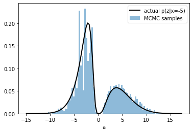
Estimate \(p(z|x_i)\) with MCMC#
num_results = 50000
num_burnin_steps = 10000
observed_x = -5
print (observed_x)
-5
# Improve performance by tracing the sampler using `tf.function`
# and compiling it using XLA.
@tf.function(autograph=False, jit_compile=True)
def do_sampling():
  return tfp.mcmc.sample_chain(
                      num_results=num_results,
                      num_burnin_steps=num_burnin_steps,
                      current_state=[
                          tf.constant([-5.], dtype=tf.float32,  name='init_avg_effect'),
                      ],
                      kernel=tfp.mcmc.HamiltonianMonteCarlo(
                          target_log_prob_fn=lambda z: scenario.zx_joint.log_prob((z, observed_x)),
                          step_size=3,
                          num_leapfrog_steps=20)
  )

states, kernel_results = do_sampling()
num_accepted = np.sum(kernel_results.is_accepted)
print('Acceptance rate: {}'.format(num_accepted / num_results))
/usr/local/lib/python3.7/dist-packages/tensorflow_probability/python/mcmc/sample.py:339: UserWarning: Tracing all kernel results by default is deprecated. Set the `trace_fn` argument to None (the future default value) or an explicit callback that traces the values you are interested in.
  warnings.warn('Tracing all kernel results by default is deprecated. Set '
WARNING:tensorflow:5 out of the last 5 calls to <function do_sampling at 0x7f971b9a7cb0> triggered tf.function retracing. Tracing is expensive and the excessive number of tracings could be due to (1) creating @tf.function repeatedly in a loop, (2) passing tensors with different shapes, (3) passing Python objects instead of tensors. For (1), please define your @tf.function outside of the loop. For (2), @tf.function has reduce_retracing=True option that can avoid unnecessary retracing. For (3), please refer to https://www.tensorflow.org/guide/function#controlling_retracing and https://www.tensorflow.org/api_docs/python/tf/function for  more details.
Acceptance rate: 0.13998
plt.plot(scenario.zr, scenario.pz_given_x(scenario.zr,observed_x), color="black",  lw=2, label=f"actual p(z|x={observed_x})")
plt.hist(states[0].numpy(), alpha=.5, bins=100, density=True, label="MCMC samples");
plt.legend()
plt.xlabel("a")
Text(0.5, 0, 'a')
Estimate \(p(z|x_i)\) with variational inference and a Gaussian class of distributions#
We want to find \(p(z|x_i)\) given a certain observation \(x_i\).
We do this by:
define a class of distributions \(Q(z|x_i) = \{q_\theta(z|x_i)\}\) parametrized by \(\theta\) hoping some distribution of this class is able to approximate \(p(z|x_i)\)
find the parameters \(w\) corresponding to the distribution \(q_w\) which is closer to \(p(z|x_i)\) in KLdiv. This is
This initially seems hard because we don’t know \(p(z|x_i)\) (which is precisely what we want to obtain), so how can be tell how any \(q_\theta(z|x_i)\) may be to it?
It turns our that the following expression is a lower bound to \(\text{arg min}_\theta\)
which is equivalent to
we choose a family of functions assuming a normal distribution for \(p(z|x)\), which may be more or less appropriate to each case.
class ApproximatePosteriorDistribution:
def get_qx(self, x_batch):
raise NotImplementedError()
def get_trainable_variables(self):
raise NotImplementedError()
def set_observed_x(self, observed_x):
self.observed_x = observed_x
return self
def set_scenario(self, scenario):
self.scenario = scenario
return self
def fit(self, batch_size=500, epochs=200):
lossh = []
optimizer=tf.keras.optimizers.Adam(learning_rate=0.05)
for epoch in pbar(range(epochs)):
with tf.GradientTape() as t:
qx = self.get_qx()
elbo_fn = lambda z: tf.math.log(self.scenario.px_given_z(self.observed_x,z)+1e-10) - ( qx.log_prob(z) - tf.math.log(self.scenario.pz(z)+1e-10))
s = qx.sample(batch_size)
loss = -tf.reduce_mean(elbo_fn(s))
gradients = t.gradient(loss, self.get_trainable_variables())
optimizer.apply_gradients(zip(gradients, self.get_trainable_variables()))
lossh.append(loss.numpy())
self.lossh = np.r_[lossh]
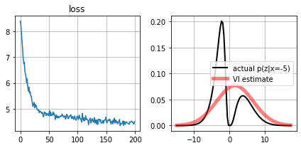
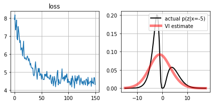
def plot_loss(self):
for ax,i in subplots(2):
if i==0: plt.plot(self.lossh); plt.title("loss")
if i==1:
qx = approximate_distrib.get_qx()
plt.plot(self.scenario.zr, self.scenario.pz_given_x(self.scenario.zr,self.observed_x), color="black", lw=2, label=f"actual p(z|x={self.observed_x})")
plt.plot(self.scenario.zr, qx.prob(self.scenario.zr), color="red", alpha=.5, lw=5, label="VI estimate")
plt.legend();
plt.grid();
class ApproximatePosteriorNormal(ApproximatePosteriorDistribution):

  def __init__(self):
      self.mu = tf.Variable(np.random.random(), dtype=tf.float32)
      self.sigma = tf.Variable(np.random.random()+1e-2, dtype=tf.float32)

  def get_qx(self, x_batch=None):
      scale = tf.math.softplus(self.sigma)+1e-5
      return tfd.Normal(loc=self.mu, scale=scale)

  def get_trainable_variables(self):
      return [self.mu, self.sigma]
approximate_distrib = ApproximatePosteriorNormal().set_scenario(scenario).set_observed_x(observed_x)
approximate_distrib.fit()
100% (200 of 200) |######################| Elapsed Time: 0:00:05 Time: 0:00:05
approximate_distrib.plot_loss()
Estimate \(p(z|x_i)\) with variational inference and a mixture of \(n\) Gaussians class of distributions#
We define
then our family of distributions is
Observe that \(\theta=\{\bar{\mu}, \bar{\sigma}, \bar{\alpha}\}\) are the parameters that will be learnt through VI.
class ApproximatePosteriorMixOfNormals(ApproximatePosteriorDistribution):

  def __init__(self, n_gaussians):
    self.n_gaussians = n_gaussians
    self.theta = tf.Variable(np.random.random(size=[n_gaussians,3]), dtype=tf.float32)

  def get_qx(self, x_batch=None):
      return tfd.Mixture(
        cat=tfd.Categorical(logits=self.theta[:,2]),
        components=[tfd.Normal(loc=ti[0], scale=tf.math.softplus(ti[1])) for ti in self.theta]
      )

  def get_trainable_variables(self):
      return [self.theta]
approximate_distrib = ApproximatePosteriorMixOfNormals(n_gaussians=5).set_scenario(scenario).set_observed_x(observed_x)
approximate_distrib.fit(epochs=150, batch_size=100)
100% (150 of 150) |######################| Elapsed Time: 0:00:11 Time: 0:00:11
approximate_distrib.plot_loss()
1
1
import torch
torch.__version__
'1.13.0+cu116'